In studying the construction of movie trailers, one of the more interesting components is figuring out how many scene changes (cuts) are included in the 2m30s of the typical trailer. While ideally one would want to match scenes from a trailer to scenes from the actual movie, we do not have access to entire movie video files. The next best thing is to use the trailer file to figure out when the video jumps between different continuous shots.
The basic logic of the process is straightforward. A video is just a collection of stills (typically 24-30 frames per second). For a continuous shot, the frame to frame differences should be “small” while a change in the shot should result in a “big” difference between 2 consecutive frames. The difficulty really lies in how to define a “small” vs “big” change in a computationally efficient way?
The first step is to understand how a computer sees a frame of a video. Suppose we have a color frame, this image is represented as a 3-dimensional (Rows X Columns X 3 colors) array. One can think of this as three 2D matrices, where each layer represents one of 3 colors (red, green, blue) and each matrix represents all the values for the corresponding color in every pixel of the frame. Each value in this 3D array corresponds to the saturation of the layer’s color. For a 24 bit (true color) image, these values range from 0 (no color) to 255 (full saturation). We can visualize the array as something like this:

Now that we know that each frame is just a simple 3D array, the difference between any 2 frames can really just be summarized by arithmetic difference of the 2 arrays. Furthermore, much of the information of the difference can be summarized by averaging the absolute (alternatively, squared) difference across the 3 layers (average absolute saturation change across RGB by pixel) and summing across all pixels. If we do this for every frame (compared to previous frame), we might visualize these differences as something like this (this is the frame to frame difference for Before Midnight – one of my favorite movies!):
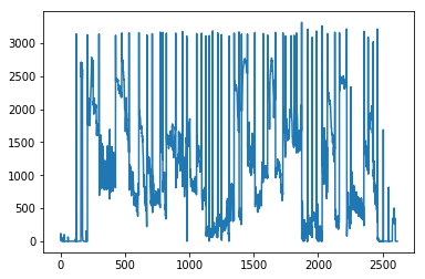
Notice, in the above figure, there are a lot of spikes followed by dense frame to frame changes that are in a locally constant-ish range. The spikes correspond to “big” differences (cuts) while the squiggles correspond to “small” differences (continuous shots). The key observation here is that the squiggles can be centered around different levels of our pixel change measure, so what we care most about is not necessarily identifying absolute cutoffs for these metrics, but rather unexpectedly high levels of the difference metric given the preceding differences within a continuous shot. In other words, we need to figure out locally “big” jumps in our frame to frame pixel difference measure.
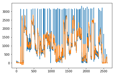
Given my recent focus on state space modeling and time series analysis (and code that I’ve already written to do this), I decided to apply those time series methods to the problem of detecting local outliers of pixel differences. Conceptually, we can use a polynomial state space model (of which a special case is the random walk + local trend model) to represent the expected evolution of pixel changes and large discrete jumps that depart from the expected range of changes should represent camera cuts. Here, we overlay the state space model predicted differences on top of the raw pixel differences graph.
Finally, we just need to look at the difference between the blue line and the orange line. Large positive differences should correspond to a camera cut. Here, the blue line represents the difference between raw and expected pixel change and we’ve demarcated scene changes with vertical red lines using a 3 standard deviation rule, i.e. if the blue difference is greater than 3 standard deviations above the expected change, we flag it as a camera cut.
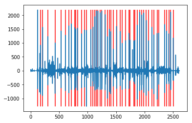
The result from these steps yields the following distinct camera cuts from the trailer. Try to match it to the video, any cuts that were missed?

